The Standardised FRTB (Fundamental Review of Trading Book)

Table of Contents

Introduction

Background

Chronology of the MR Changes

Shortcomings

A Clearer Distinction

       The Trading Based Boundary

Valuation based Boundary

Common Changes

Valuation Risk Assessment

Calculation Frequency

Key FRTB Elements

Internal Model Based Eligibility

In Summary

Standardised Approach

Alignment to Internal Model Methods

 

 

 

 

 

Introduction

The Basel Committee published in May 2012 a consultation paper proposing a more robust boundary between Trading and Banking books to avoid regulatory arbitrage, capture market illiquidity more effectively, strengthen the risk measurement and valuation requirements under both standardised and internal model based approaches along with strengthening the relationship between the two approaches.

Background

The 2008 crisis highlighted the severe undercapitalisation of the trading book exposures. This characteristic was to a large extent the result of the risk measurement and valuation methodologies used by banks.

The crisis exposed a series of fundamental weaknesses of the overall design of the trading book regime which contributed or amplified the impact of the crisis.

Basel 2.5 introduced some changes but they were recognised to be insufficient.

Chronology of the MR Changes

1995	Internal Model Based approach to MR VaR
2009	Stressed VaR
	Standard Rules
	IRC
	CRM (Comprehensive Risk Measure)
	CVA
	Risk not in VaR and Stressed RNiV
2017	FRTB

Shortcomings:

Consistency and Coherence: there is no consistent view of risk categorisation and capitalisation

Tail Risk: Not consistently or fully captured

Market Liquidity Risk: Not consistently or fully captured

Bank-Specific variability: Supervisory multiplier, historical window length, weighting scheme, scaling, aggregation

Pro-cyclicality: risk measures and capital increase as economic conditions worsen

Overalapping of models: double counting VaR, SVaR, IRC

Hedging and diversification: Benefits from using these techniques are overstated

 

A clearer distinction

The BIS proposed to reconsider what constitutes an asset in the TB and BB.
The initial distinction was dictated by the bank’s intent to hold an asset for trading purpose or to hedge a position held for trading purposes. Prior to FRTB, the boundary between TB and BB was subject to regulatory arbitrage giving rise to lightly capital charged trading books.

The BIS proposed two alternative definitions:

1. A trading evidence based boundary
2. A valuation based boundary

 

The trading evidence based boundary

Unlike the existing boundary the trading evidence based boundary is designed to be objective. The trading evidence is based on the trading intent, hence inclusion of trades in the TB requires proof of such intent.

Such proof may be the product of statistics on the position turnover, rebalancing frequency for their hedges and their average age. Banks would be required to produce evidence of the feasibility of trading an instrument. This now includes proofs of access to relevant markets for trading and hedging, owning historical data and market data for the underlying and a plausible plan to justify why and how the bank would trade on a market in which it had limited experience.

Banks would also be required to demonstrate active management of trading positions ad to do so they may need to set and enforce limits both on an instrument and on a risk position basis. Another new requirement would be for banks to actively monitor market liquidity levels (including market data records) and to specify an expected maximum holding period for an instrument with penalties if that period is exceeded.

The Valuation Based Boundary

This approach would dispense altogether with trading intent and instead apply market risk capital requirements to all fair valued financial instruments for which valuation changes could lead to a reduction in a bank’s capital resources.

This would significantly increase the size of bank’s TB and increase the number of banks subject to market risk capital requirements. In accounting terms the new TB would include held for financial instruments, available for sale financial instruments and other financial instruments to which fair value is applied either as an option or a requirement.

Common Changes

Regardless of which of these boundaries is finally adopted, the proposal includes some common changes:

1. Banks will be subject to more stringent public disclosure requirements regarding their trading positions
2. Banks will be restricted from changing the book destination. This limitation is imposed by the trading evidence based boundary or through the fair value accounting requirements in the valuation approach
3. All fair valued financial instruments either in the TB or BB will be subject to more specific stringent prudent valuation requirements.

New Approach to Risk Assessment

In addition to the new boundaries the committee has proposed a series of changes designed to make the market risk calculation more risk sensitive.

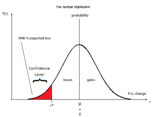
1. BIS proposed to replace the VaR risk metric with a new ES method (Expected Shortfall). ES considers a broader range of potential outcomes than VaR and measures risk by considering both size and likelihood of losses above a certain confidence level. ES is expected to capture the tail risk (the risk of unforeseen events not factored into a bank’s VaR model)
2. BIS proposes to recalibrate the TB framework such that market risk capital charges are sufficient not only in benign market conditions but also in periods of stress.
3. The Committee is moving away from the assumption of market liquidity which was central to the market risk framework prior to the financial crisis. The Paper proposes to incorporate market illiquidity risks as an integrated component of the market risk framework. To achieve this, it proposes three key changes designed to capture market illiquidity at a bank-specific and market-wide levels:
   a) Market liquidity would be assessed using the concept of “liquidity horizons” –which is the time required to exit or hedge a risk position in a stressed market without materially affecting market prices;
   b) “endogenous” liquidity risk that might imply that the cost of unwinding portfolios might be affected by the bank’s own trading behaviour or other idiosyncratic factors should be accounted for by further increasing liquidity horizons;
   c) banks would be required to hold capital for potential future jumps in liquidity premia for instruments that could become particularly illiquid under stressed conditions (captured on a forward looking basis)

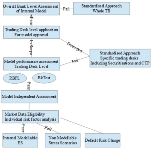
Calculation frequency

Market Risk capital will be required to be calculated daily at trading desk level. Approval to use internal models is to be assessed daily at same level using two new tests:

1. Back testing
2. P&L attribution

The trading desks that fail any of the above tests will need to be capitalised under the Standardised method , also known as Sensitivity Based Approach. Trading desks that pass both tests will be capitalised using the firm’s Internal Models.

As already mentioned, ES will replace the VaR whilst Incremental Default Risk will replace the Incremental Risk Charge. Time series data will also be subject to quality assessment.

Key FRTB elements

Liquidity Modelling	Eligibility	Capital Calculations
Stricter Data Requirements	TB vs BB Boundary	Capital Aggregation
Granular Trading Desk level focus	Model Backtesting	Internal Model (ES)
Conservative treatment of hedging and diversification	RBPL	Non Modellable Stress Scenarios
Tail risk capture	Leverage Ratio	STD Approach
Increased granular disclosure requirements	Market Data Eligibility	Incremental Default Risk
Coherent approach
Consistent treatment of credit risk

Internal Model Based Approach Eligibility

Banks will be allowed to use one of the two available methodologies to calculate capital under the new rules: Standardised or Internal Model

In Summary

FRTB concerns with new rules to determine the scope of the instruments eligible for inclusion in the TB.

There are now more stringent requirements governing internal risk transfer between the BB and the TB.

The introduction of the Liquidity Horizons in the 97.5% ES calculation is to reflect the period of time required to sell or hedge a given position during a period of stress.

The replacement of VaR and Stressed VaR with a single expected shortfall risk measure aims at capitalising for the loss event in the tail of the P&L distribution.

Back testing requirements of internal models at trading desk level will determine the validation of the models in use. Should backtesting fail, the trading desk will have to apply the standardised approach.

The replacement of the IRC with a Default Risk Model, aims at capturing the default risk in the market risk framework.

The revised Standardised Approach for market risk is now based on price sensitivities, therefore more risk sensitive. BIS intention to set up the new STD approach was to reduce the gap with the Internal Models results.

Public disclosure on market risk capital charges under STD and Internal Models is now enhanced.

 

Standardised Approach

Under the existing framework, there are material differences between the Standardised and Internal Models based methodologies. The current standard rules are based on a simple Risk Weighted and Notionals or Mark to Market based Approach.

Banks in the past have been criticised for overusing the internal models in order to achieve lower capital requirements. The current Standard methodology did not allow for wide diversification and hedging benefits. The new framework would provide a method for calculating capital requirements for banks without sophisticated measuring model in place and would ensure a more appropriate fall back calculator should the Trading Desk fail the internal model eligibility test.

Alignment to Internal Models Method

The new Standard Rules are more aligned to the Internal Models Method in terms of capital requirements. Instruments are now bucketed as per their risk characteristics. The Risk Weights of each bucket are prescribed and they have been calibrated with the internal models for Expected Shortfall. There is now more recognition of hedging and diversification benefits through the use of an aggregation formula using the regulatory prescribed correlation parameters.

Standardised Capital Charge Calculation Process Flow

The STD capital requirement is the sum of:

Enhanced Delta Risk Capital Charge + Default Risk Capital Charge + Residual Risk Add On

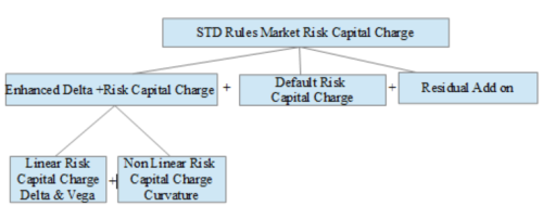
Banks are required to calculate the ‘Enhanced delta plus Risk’ and ‘Default Risk’ capital charge at the following portfolios levels:

1. Complete trading desks
2. Non Internal Model Approach (Desks which failed the model eligibility tests)
3. Each desk as a portfolio on its own: no diversification or hedging benefits across desks

Delta, Vega and Curvature

The Basel Committee decided to implement the “enhanced delta plus method”, which is sensitivity-based, differentiating between three different risk components: delta risk as a foundation for capturing linear risks, and vega and curvature risk as two additional components which apply to products with optionality.

Vega risk assesses the risk of price changes based on market expectation on future volatility. In other words the sensitivity to the volatility.
Curvature risk captures the non-linear risk, which is not accounted for by delta risk.

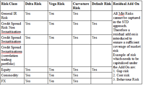
STD Risk Class Definitions

Sensitivities are calculated for 7 Risk Classes in STD approach:

1. GIRR
2. Equity
3. Credit Spread Securitisations
4. Credit Spread Non Securitisations
5. Credit Spread Securitisations Non Correlation Trading Portfolios
6. Commodity
7. FX

The STD capital charge is also calculated on the above risk classes according to the relevant sensitivities: Delta, Vega, Curvature and Default Risk

The linear and non linear capital charges are calculated separately with no diversifation benefit recognised between them.

Options are subject to Vega and Curvature risks.

More specifically for each Risk Class:

Risk Class	Sensitivity	Risk Factor
General IR risk	Delta	Defined along two dimensions: 1) A risk-free yield curve for each ccy in which IR sensitive instruments are denominated 2) Vertices (maturity points): 0.25, 0.5, 1, 2, 3, 5, 10, 15, 20, 30 Also includes inflation and cross currency basis risk factors. (Delta is the rate of change of the theoretical option value with respect to changes in the underlying).
	Vega	Vega Rf are the implied volatilities of options that reference GIRR sensitive underlyings defined along two dimensions. (the Sensitivity to Volatility) 1) Maturity if the option mapped to the vertices :0.5, 1, 3, 5, 10 yrs
	Curvature	Defined along only one dimension: the constructed risk free yield curve per currency
Credit Spread Risk Non Sec.	Delta	Defined along 2 dimensions 1) the relevant issuer credit spread curves (Bond and CDS) 2) Vertices: 0.5, 1, 3, 5, 10 yrs
	Vega	The Vega Rf are implied volatilities of options that reference credit issuer names as underlyings (bonds and CDS). Further defined along maturity of the option mapped to the vertices: 0.5, 1, 3, 5, 10 yrs
	Curvature	The relevant issuer credit spread curves (Bond an CDS)
Credit Spread Risk Sec.	Delta	Rf are defined along 2 dimensions: 1) the relevant tranche credit spread curves 2) Vertices: 0.5, 1, 3, 5, 10
	Vega	Vega risk factors are the implied volatilities of options that reference non CTP credt spreads as underlying (bond and CDS) defined along maturity of the option mapped to the vertices: 0.5, 1, 3, 5, 10
	Curvature	The relevant tranche credit spread curves (Bond and CDS)
Credit Spread Sec (Correlation Trading Portfolio)	Delta	Risk factors are defined along two dimensions: 1) The relevant tranche credit spread curves 2) Vertices: 0.5, 1, 3, 5, 10
	Vega	Vega rf are the implied volatilities of options that reference non CTP credit spreads as underlyings
	Curvature	The relevant tranche credit spread curves (bonds and CDS)
Credit Spread Risk Securitisaitons (correlation trading portfolio)	Delta	Defined along two dimensions: 1) the relevant underlying credit spread curves (bonds and CDS) 2) Vertices: 0.5, 1, 3, 5, 10
	Vega	Vega rf are the implied volatilities of the options that reference CTP credit spreads as underlyings (Bonds and CDS) defined along maturity and the option mapped to the vertices: 0.5, 1, 3, 5, 10
	Curvature	The relevant underlying credit spread curves (bond and CDS)
Equity	Delta	Either: 1) Equity Spot prices 2) equity repo agreement rates
	Vega	The implied volatilities of the options that reference the equity spot prices as underlyings along maturity of the option dimension at the 0.5, 1, 3, 5, 10 yrs
	Curvature	Equity Spot prices
Commodity	Delta	Commodity spot prices depending on the contract grade of the physical commodity and time to maturity of the traded instrument
	Vega	The implied volatilities of the options that reference commodity spot prices as underlyings along maturity of the option dimension at the 0.5, 1, 3, 5, 10 years
	Curvature	Commodity spot prices
FX	Delta	All the exchange rates between the currency in which an instrument is denominated and the reporting currency
	Vega	The implied volatilities of the options that reference exchange rates between currency pairs with maturity of the option defined at the vertices 0.5, 1, 3, 5, 10
	Curvature	All the exchange rates between the currency in which an instrument is denominated and the reporting currency

Sensitivities Definition for STD approach

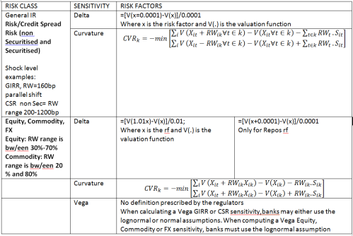
Linear Capital Charge Calculation under the STD approach: DELTA

Linear Capital Charge is calculated for each risk class separately. The Delta sensitivity is 1bp absolute in GIRR and CSR risk factors, or 1% relative move in EQ, FX and Comm Risk Factors.

The positions in a risk class are placed in buckets defined per risk class. Each bucket has a predefined RW. For example, Equity buckets are defined along 3 dimensions: region, market capitalisation and industry.

Net the sensitivity Sk across instruments to each risk factor k belonging to the same bucket. The Sensitivities cannot be netter across buckets

Calculation of the Risk Weighted net sensitivities follows: WSk=RWksk

In each of the buckets ‘b’, aggregate the weighted sensitivities across risk factors using the following:

 

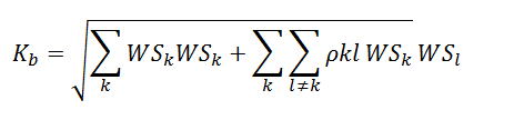
The correlation parameter pkl between risk factors have been prescribed by the BIS. TO come up with delta capital charge for a risk class, bucket level capital Kb is aggregated as follows:

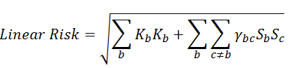
The Basel Committee prescribed similarities for across buckets aggregation, correlation parameter Ybc, between buckets for each risk class

Linear Capital Charge Calculation under the STD approach: VEGA

Calculation of Vega capital charge remains the same except for RW, correlations and sensitivity calculations. The RW used in Vega is calibrated to each risk class liquidity horizon and is not dependent on the bucket structure as Delta capital charge was.

Vega is defined along the option maturity at 5 tenor points. Hence, Vega of a position with a given maturity has to be allocated to one or two of the 5 tenor points.

Example:

Suppose an equity call option position with Vega of 100 and maturity of 4.5 years.

Vertices or maturity points are 0.5, 1. 3. 5. 10 years.

The position is linearly allocated between 3 and 5 years.

At yr 3 vertice, allocate 100*{(5-4.5)/(5-3)}

At yr 5 vertice, allocate 100 * {(1-[(5-4.5)/(5-3)]}

Vega sensitivity is calculated as a product of the option Vega as allocated above and its implied volatility at the relevant maturity tenor.

The BIS has prescribed the method to calculate the correlation parameter: one for the GIRR and another for the other asset classes.

Non-Linear Capital Charge Calculation under the STD approach: Curvature

Curvature capital charge calculation follows the same buckets and risk class foundations of linear capital charge with the only difference that this sensitivity is calculated by applying a stress move to the risk factor

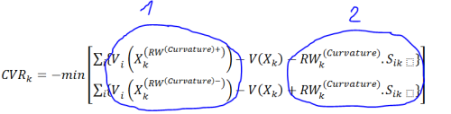
from the above equation:
in 1. the risk factor is shocked equivalently to the RW of the bucket in which the position is placed. In 2. we strip the delta from the curvature sensitivity to avoid double counting.

The correlation parameters in the intra bucket and across bucket aggregation formulas are the same as those used in the delta capital charge calculation.

Example:

Suppose we have an option on IBM stock. (Large market capitalisation, Advanced economy, Technology, Bucket 8, RW 50%). Current Stock Price is USD 151.31

The stock price is bumped to USD 227.01 (151.341.5) and USD 75.67 (151.340.50). The position are revalued at the above stock market price level holding other risk factors constant.

The Curvature is  calculated as:

CVR+= (227.01-151.31)-(Δ*RW)

CVR-= (75.67-151.31)+(Δ*RW)

CVR= min(CVR+, CVR-)

The FO system will ahve to provide the valuation for a position in the 2 scenarios and current price. Curvature is then calculated for the capital charge.

Default Risk Charge

Prior to FRTB, banks capture default and migration risk using the models for securitised and non securitised portfolios.

Namely: IRC for non Securitised Portfolios and All Price Risk (APR) or Comprehensive Risk Measure (CRM) for Securitised Portfolios (correlation trading portfolios).

The above are model based approaches, therefore no Standard default risk calculation exists except for securitisations trades. Default risk does not apply to equity portfolios either.

Going forward the standardised default risk charge will be calcualated for all trading desks in scope.

The capital requirement for default risk is the sum of the default risk of:

non-securitisations (including equity), Securitisations (non correlation trading portfolio) and Securitisations (correlation trading portfolios).

The DRC captures the Jump-To-Default risk at 1 year horizon and it’s calibrated  on the basis of the banking book credit risk treatment in order to reduce the potential discrepancy in capital requirements for similar exposures in the Banking Book.

Similar to the enhanced delta plus component of the STD approach, it allows some hedging recognition at a bucket level.

The calculation steps are:

1. Categorise positions as long or short (a long position implies the default of the underlying obligor results in a loss)
2. Positions are assigned a seniority on the basis of the allocated LGD
3. Gross JTD is calculated  per position. This value is a function of the LGD, notional amount (face value) and the cumulative P&L already realised on the position
4. Scaling and offsetting is performed on gross JTD to arrive at net JTD
5. Underlying obligors ratings are assigned in each of the net JTD position and placed in the defined buckets
6. Calculate hedge benefit ratio for each bucket
7. Calculate DRC for each bucket
8. Calculate total capital charge for DRC by sum of bucket level capital charges
9. No hedging or diversification is recognised across buckets in any given scope

 

Residual  Risk Add On

The objective of this charge is to capture the risk which is not covered by the Enhanced Delta Plus Risk and Default Risk.

The scope of this add on is any instrument satisfying both conditions below:

1. It is subject to Vega Sensitivity and Curvature capital charge in the Trading Book
2. Its pay off cannot be written as a linear combination of vanilla options

An example of instruments affected by residual risk add on are path dependent options.

The Add On calculation is straightforward:

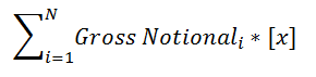
N= total number of positions under scope

x = the add on multiplier (1% is the prescribed value)

Gross Notional is the notional amount of the instrument i. 

In case the Notional amount is unavailable, then the maximum potential loss should be used.

General Interest Rate Risk Class Buckets and respective Risk Weights

Tenor	0.25Yr	0.5Yr	1Yr	2Yr	3Yr	5Yr	10Yr	15Yr	20Yr	30Yr
RW	1.6%	1.6%	1.5%	1.25%	1.15%	1.0%	1.0%	1.0%	1.0%	1.0%

Credit Spread Risk Non-Securitised/Securitised Correlation Traded Portfolios Risk Class Buckets and respective Risk Weights

Bucket	Credit Quality	Sector	RW
1	Investment Grade	Sovereigns, CTRL banks, Multilateral Dev Banks	2.5%
2		Financial including Gov backed financials	5%
3		Basic materials, energy, industrial agriculture, manufacturing, mining and quarrying	3.5%
4		Consumer Goods and Services, Transportation and Storage, Admin and support  service activities	3%
5		Technology and telecom	2.5%
6		Health Care, utilities, Local Govt, Gov-backed non financial, education, public admin, professional and technical activities	2%
7	High Yield and  Unrated	Sovereigns, CTRL banks, Multilateral Dev Banks	10%
8		Financial including Gov backed financials	12%
9		Basic materials, energy, industrial agriculture, manufacturing, mining and quarrying	9%
10		Consumer Goods and Services, Transportation and Storage, Admin and support  service activities	10%
11		Technology and telecom	9%
12		Health Care, utilities, Local Govt, Gov-backed non financial, education, public admin, professional and technical activities	6%
13	Other Sectors		12%

Credit Spread Risk Securitised Non-Correlation Traded Portfolios Risk Class Buckets and respective Risk Weights

Bucket	Credit Quality	Sector	RW
1	Senior Investment Grade	RMBS Prime	4%
2		RMBS Mid Prime	6.5%
3		RMBS Sub Prime	8.5%
4		CMBS	8.5%
5		ABS Student Loans	3.5%
6		ABS Credit Cards	5%
7		ABS Auto	5%
8		CLO Non-CTP	6%
9	Non-Senior Investment Grade	RMBS Prime	8%
10		RMBS Mid Prime	13%
11		RMBS Sub Prime	17%
12		CMBS	17%
13		ABS Student Loans	7%
14		ABS Credit Cards	10%
15		ABS Auto	10%
16		CLO Non-CTP	12%
17-24	High Yield and Unrated	Same buckets as above	The RW for the buckets 17-24 are then equal to the corresponding RW for the buckets 1 to 8 scaled up by a multiplication of 4
25	Other Sector		34%

Equity Risk Class Buckets and respective Risk Weights

Bucket	Market Cap	Economy	Sector	RW
1	Large Market Capitalisation ≥USD2bn	Emerging Market Economy	Consumer Goods and Services, Transportation and Storage, Admin and Support Service activities, healthcare, utilities	55%
2			Telecom and  Industry	60%
3			Basic materials, energy, agriculture, manufacturing, mining and quarrying	45%
4			Financials including Gov backed financials, RE activities, technology	55%
5		Adv Economy CAN, USA, MEX, €zone, non €zone, JAP, AUS, NZL, SIN, HK, SAR	Consumer Goods and Services, Transportation and Storage, Admin and Support Service activities, healthcare, utilities	30%
6			Telecom and  Industry	35%
7			Basic materials, energy, agriculture, manufacturing, mining and quarrying	40%
8			Financials including Gov backed financials, RE activities, technology	50%
9	Small	EM	Same as above	70%
10		ADV Economies	Same as above	50%
11	Residual			70%

Commodity Risk Class Buckets ad respective Risk Weights

Bucket	Commodity Category	RW
1	Coal	30%
2	Crude Oil	35%
3	Electricity	60%
4	Freight	80%
5	Metals	40%
6	Natural Gas	45%
7	Precious Metals (+ gold)	20%
8	Grains and Oilseed	35%
9	Livestock and Dairy	25%
10	Softs and other Agric	35%
11	Other Commodities	50%

FX Risk Class Buckets ad respective Risk Weights

The Bucket structure is defined by each currency pair. (one bucket = one currency pair)

The FX weight  is fixed at 15% and applied to all sensitivies  or risk exposures. However for the following currency pairs, the 15% RW is divided by the SQRT of 2.

USD/EUR, USD/JPY, USD/GBP, USD/AUD, USD/CAD, USD/CHF, USD/MXN, USD/CNY, USD/NZD, USD/RB, USD/HKD, USD/SGD, USD/TRY, USD/KRW, USD/SEK, USD/ZAR, USD/INR, USD/NOK, USD/BRL, EUR/JPY, EUR/GBP, EUR/CHF, JPY/AUD

The Internal Model Approach (IMA)

Current VaR

To calculate portfolio VaR,  Portfolio mean & Portfolio standard deviation (which includes effect of correlation between each individual security in the portfolio) is used, thus when  Portfolio VaR is calculated, it would always be equal or less than the aggregate VaR of each individual security in the portfolio, which satisfies the subadditivity criteria.

Expected Shortfall

The Expected Shortfall behaves differently. ES is sub-additive giving more diversification benefits. Under ES estimation the tail region is assigned a distribution(e.g. extreme value) now this distribution is divided into equal probability slices weighted by the more general risk aversion (weighting) function. The focus is on tail region only the difference is that the tail region itself follows a distribution which is then treated as said above to estimate the ES. It is generally assumed to be difficult to backtest and implement for the lack of peers and simulate through Montecarlo. ES is calculated using the instantaneous shocks equivalent to the movement of the relevant Risk Factors during the time span associated to the liquidity horizon. The risk factor move is taken from the 12 more stressful months since 2005.

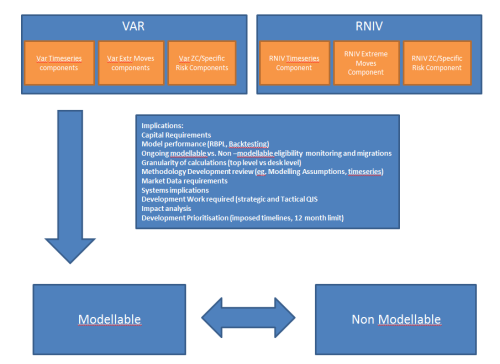
Affected calculators

The key changes affects the calculations of the following:
a) Internal Models (non modellable component), b) Standard Rules, c) Incremental Default Risk, d) Default Risk Charge and e) Capital Aggregation.

Methodology inputs are common to all of asset classes

Current	FRTB
VaR	NA
Stressed VaR	Stressed Expected Shortfall

99% VaR

Internal Model Approach: Liquidity Horizons

Liquidity Horizon is the time required to execute a transaction and liquidate the position in stressed market periods  The increase in Liquidity Horizons from the previous 10 days to the the actual 250 is also another major change.

Before the increase of the Liquidity Horizon values, the market believed that trading book positions could be easily sold or hedged in the in the market over 10 day holding period.  This was not what really happened. BIS proposed to incorporate the liquidity horizons into the market risk metrics similarly to the IRC and CRM (comprhensive risk measure)

Banks risk factors are now assigned 5 LH categories (IR, Equities, FX, Credit Spreads and Commodities):

Risk Factor Category	Liquidity Horizon
IR	20
IR ATM volatility	60
IR (other)	60
Equity Price (large Cap)	10
Equity Price (Small Cap)	20
Equity Price (Large Cap) Volatile	20
Equity Price (Small Cap) Volatile	120
Equity (Other)	120
FX Rate	20
FX Volatility	60
FX (other)	60
Credit Spreads	20-250
Commodities	20-120

Credit Spreads: capital requirements increase disproportionately to to other asset classes. Some Liquidity Horizons categories seem arbitrary: US treasury and USD/EUR FX have double the liquidity horizon compared to Large Cap Equity (10 days). It’s difficult to interpret and analyse the results. In addition, operational challenges are substantial.

In addition,

ES is calculated using instantaneous shocks equivalent to the movement of the risk factors during the time span of the associated liquidity horizon. ES ignores dynamic re-balancing and trades maturity and the path dependency. In fact it’s risk factor dependent not product dependent. In addition, ES is independent of the position size.

A LH class is assigned to each sensitivity position and passed on to the P&L component (P&L Strips). This attribute is used for bucketing and aggregation of P&L Strips for the purpose of calculating the cascading expected shortfall and to calibrate the stressed scenario shocks for non modellable components.

Liquidity Horizons Implementation Approach

There are two versions of Liquidity Horizons methodologies:

1. Full LH implementation Approach
2. Scaling LH approach

Full LH implementation

The Full LH implementation approach requires the following:

• Calculation of the moves/shocks in the time series over various LH depending on the risk factor (10, 20…250 days)
• Calculation of the corresponding P&Ls
• Aggregation of the PL st;rips aligned by start date

The Pros of this approach are:

• Actual underlying market moves
• More accurate for long horizons (not exceeding theoretical limits)
• Recognition of barrier effects (knock in, knock out) in partial/full reval models

The Cons of this approach are:

• Difficult to implement
• May violate non-arbitrage conditions causing pricing models to fail
• Large overlapping periods
• Distorts correlations b/ween asset classe
• Does not recognise hedging/re-hedging benefits as different risk factors are shocked by different LHs

Scaling LH Approach

The scaling approach is deterministic and driven by a formula

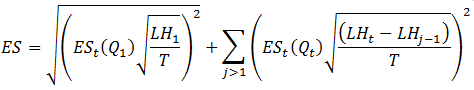
ESt is the Expected Shortfall at horizon T (days)

Qj is the subset of risk fators whose liquidity horizons are at least as long as LHj

The Pros of this approach are:

• Easy to implement based on existing 10 days P&L strips
• Retains correlation structures

The Cons of this approach are:

• Scaling P&L rather than market moves introduces additional errors, ignoring non linearity
• Squareroot time  scaling assumes IID returns, not always valid
• May break theoretical parameters limit
• Does not recognise hedges/re-hedging as different risk factors are shocked by differnet LHs
• Does not recognise barrier effects

Constraints on diversification benefits

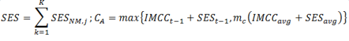
FRTB ES Aggregation

Two approaches are possible:

1. Unconstrained: It calculates ES allowing diversification effects between risk factor classes (full correlation benefit)
2. Constrained: It calculates ES without diversification effects between risk factor classes (correlation benefit only within asset classes)

Capital_modellable= p Unconstrained + (1-p)Constrained

where p is determined by the regulators post QIS

Expected Shortfall – Capital Uplift Drivers

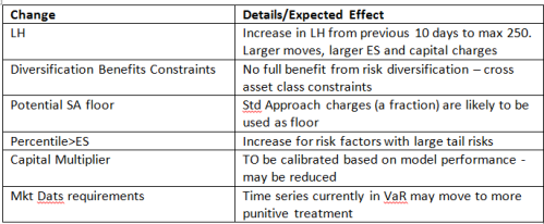
Non Modellable – Stress Scenarios

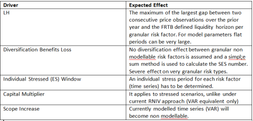
Implications:
Punitive capital charges, more conservative than other approaches, including:

• Current RNIV approach (PRA) where diversification within risk types is recognised
• Standard rules framework where diversification between offsetting trades in neighbouring buckets are allowed.

Examples

IR Volatility Skew

Currently:

• RNIV is to be included in VaR soon via timeseries simulation
• Risk is captured via sensitivities and timeseries to the SABR volatility model parameters (ALpha, Beta, Rho)
• Parameters are not very frequently marked but data is filled using stochastic bridges
• Using historical simulation, there is a great deal of offsetting betwenn the P&L strips for each risk factor

FRTB treatment:

• The actual marks do not satisy the FRTB requirements criteria
• Bridged data points are not real prices and cannot count as observations
• THe IR Vega Skew will be considered as non-modellable (>96&) and will be capitalised via stress scenarios

Effects:

• Breakdown P/L strips into 5832 stress scenrios (18 tenors*18 expiries*3SABR parameters*6 currencies)
• LH driven by largest gaps/flat periods in data (IR Vega LH floor)
• Stressed period specific to each risk factors
• Overall RWA uplift factors > 20 X current RNIV VaR

Drivers:

• Reducing grnularity of grids to 10X10 (STD Granularity) results in ~25% RWA reduction
• Allow aggregation across expiries and only consider tenors as risk factors ~60% reduction
• Allow diversification benefits via IR Vega STD Approach correlations ~65% reduction

Potential Mitigation

• Regulatory feedback and consultation
• Ensure SABR parameters are marked at least 24 times a year with no gaps longer than a month

 Regression Models (RNIV)

Currently:

• Regression models capture market risk via a weighted average (index) timeseries (XBeta)
• Specific risk is captured via extreme moves (regression residual)
• 10 Day moves/shocks are used
• Specific risk components are aggregated using zero correlation

FRTB treatment if non-modellable:

• Every issuer/single name is shocked by Expected Shortfall shock corresponding to its own worst year
• Conservative aggregation by absolute sum
• Zero correlation to absolute sum (SQRT (N) uplift factor where N is the number of single names/issuers (N~1000s)
• LH driven shocks is the largest gap in own data, prescribed asset class LH floor

Potential migration:

• Improve data and include in modellable where possible
• RNIV examples: Borrow cost (single names), ETF NAV vs Listed Basis, EQ VEga Skew Convexity

Non Modellable – Specification of market risk factors

Risk factors Vs Pricing Inputs definition: Factors that are deemed relevant for pricing should be included as risk factors in the bank’s internal models. Where a risk factor is incorporated in a pricing model but not in the risk capital model, the bank must justify this omission to the satisfaction of its supervisor.

Additional risk will be in scope (basis risk) to ensure model performance with regards to:

1. Backtesting (capital multiplier impact)
2. P&L attribution

Model parameters

• Scope: inclusion in line with the current trends imposed by the regulators
• Check if the model dependent parameters are real prices
• Minimum data requirements are 24 observation with maximum 1 month gap and check if observation gaps and flat periods differ
• Offset with valuation reserves
• Granularity of parameters (IR Skew and Correlation risks) currency, tenor, maturity attributes grids, marked at the same value, existing offsetting RNIV will not be realised

Possible unforeseen consequences

• Dis-incentivise hedging of illiquid risks (trade and hedge offset is not recognised
• Dis-incentivise the development of more complex and more flexible risk models where dta fails the frequency and real price test
• Incentivise retrenchment of efforts to increase risk factor granularity over the past 5 years (move from 20 to the minimum of 6 tenor buckets (min imposed) to avoid significantly larger capital charges.

Modellable/NonModellable vs RNIV

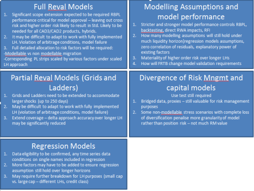
Review of the common Risk Models in Investment Banking

Incremental Default Risk

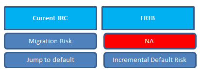
Consistent Treatment

The potential MtM loss from shocks to credit spreads (including Migration risk) will be captured by the ES models of price risks

IDR models where the loss is incremental to the risk already captured in the ES price risk model

Key Points

• A 1 yr time horizon calibrated to a 99.9th percentile confidence level
• correlaiton parameters must be estimated based on listed equity prices and use a one year observation period based on a period of stress
• PD floor is 0.03%
• two factor simulation model
• Joint approval process with credit spread risk